|
Hertzsprung-Russell diagrams In July’s WMA webinar, we looked at Hertzsprung-Russell diagrams. H-R diagrams are one of the most important tools available in stellar physics, since they indicate a great deal about the characteristic of stars. The H-R diagram below, known as a theoretical H-R diagram, is a scatter plot of stars photosphere temperature vs. luminosity. Brian Davidson’s last couple of Blogs have mentioned the Summer Triangle asterism, consisting of Vega, Deneb, and Altair. Taking a sample of ‘nearby stars’ as shown below we have marked the Summer Triangle stars on the H-R diagram, showing how different these three stars are: 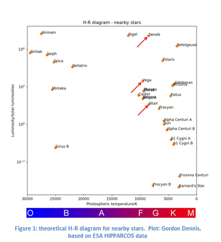 The spectral classes of the stars are indicated by the familiar ‘OBAFGKM’ legend. Before looking at the three stars, look at the track running from Alnitak at the top left to Proxima Centuri at the bottom right. This track is the Main Sequence, where in the stars interior hydrogen is converted into helium by nuclear fusion. Stars leave the main sequence once about 11% of the hydrogen-mass has fused to helium and the core of the star becomes unstable. About 90% of stars are on the main sequence. It may not appear like this from the diagram, but that’s because of our sample, which is ‘nearby stars’. Altair is a main sequence star, larger and hotter than the Sun. It will therefore have a shorter main sequence life than the Sun. Altair’s luminosity is 10.6 L⊙. Recall that luminosity is a measure of the power radiated by a star; the unit of luminosity is the Watt. Vega has a photospheric temperature similar to that of Altair. But Vega’s hydrogen burning phase is now over. The star has entered the main sequence turnoff, on the way to becoming a red giant, before shedding its outer layers to form a planetary nebula. At that time, what will remain of Vega is a hot white dwarf star at the bottom left of the H-R diagram. This sequence of events will also be what happens to the Sun when main sequence turnoff occurs. Deneb is a super-giant star. Although Deneb’s Photospheric temperature is comparable to both Vega and Altair, its luminosity is very much greater. Deneb has a luminosity of more than 104 L⊙, a mass of 19M⊙ and is destined to end its life in a Type II supernova event. This will leave a supernova remnant perhaps like the Crab Nebula, M1 and a neutron star which is way off scale at the bottom of the H-R diagram. Open clusters and globular clusters For this month’s Blog, we’ll consider a question asked at the July WMA webinar, “Can we make H-R diagrams of star clusters to help determine their characteristics?” The answer is yes. Astronomers are familiar with both open clusters and globular clusters. Their main characteristics are shown in the table below. 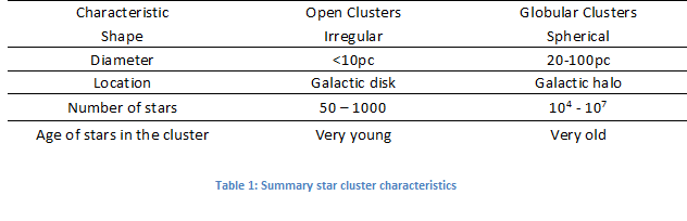 How can we conclude that open clusters consist of young stars and globular clusters consist of old stars? The amount of hydrogen that a star has available for fusion is directly proportional to the star’s mass. In simple terms, the greater the mass of hydrogen packed in, the faster the reaction rate, and the higher the luminosity. The star’s luminosity determines how quickly the star will fuse the hydrogen into helium, and hence how long the star lives on the main sequence according to the relation:  Since from the mass-luminosity relation we know that:  Substituting 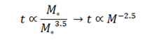 The diagram below summarises how stars of different spectral classes leave the main sequence - the “main sequence turnoff” - as they evolve: 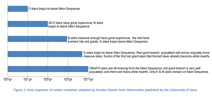 Plugging the numbers into the equations, this means that a star of 10M⊙ will have a lifetime of only about 13 million years. Bear in mind that we know that about 80% of stars are red dwarfs, smaller than the Sun. A low mass star of about 0.6M⊙ has a life of ~34 billion years. That time is much greater than the age of the universe which means that no low mass star has yet completed its main sequence lifetime. H-R diagram for open cluster M45 So, let’s plot an observational H-R diagram, (also known as a “colour-magnitude diagram”) for open cluster M45, known of course as the Pleiades: 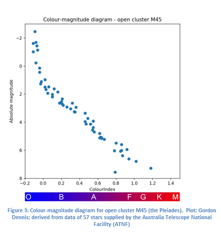 The observational H-R diagram above is a plot of absolute magnitude (VMag) vs. colour index (BMag-VMag). The scale ranges are (x: colour index 0.2 à 1.45; y: absolute magnitude 8 à -2) . We can see at the top left of the H-R diagram, only a few of the larger, more luminous (which of course implies more massive) stars in the Pleiades have begun their main sequence turnoff. These are the dots at the top left which are turning upward and to the right. The majority of the (less massive) stars in the plot remain very much on the main sequence. They are so young that hydrogen burning has a while to progress. It is generally thought that open clusters disperse after a short time (in cosmological terms) before the stars in them have commenced main sequence turnoff. It is also thought that then Sun formed in an open cluster which subsequently dispersed and that this accounts for the fact that the Sun is isolated and not part of a multiple star system, although that is far less certain. H-R diagram for globular cluster M14 Now, let’s look at the H-R diagram for globular cluster M14. This H-R diagram is markedly different to that of M45. The plot is a subset of the total data of over 1,000 stars and is plotted with the same scale ranges as the M45 plot. 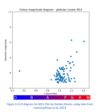 In the M14 H-R diagram, just about no main sequence stars are evident. The reason is that most stars in M14 are very old, and have completed hydrogen burning and moved off the main sequence. Low mass stars are either ascending the red giant branch or have already become red giants. Like Altair, Vega, and the Sun, they will end their lives as white dwarfs. A few at the top right of the H-R diagram are supergiants and, like Deneb, will finish their lives in Type II supernova events.
The fact that the majority of stars in this globular cluster are grouped at the red end of the colour index confirms the generally red appearance of the globular cluster. References Data sources Contreras Pena, C et al (2013). The globular cluster NGC6402 (M14). A new BV color-magnitude diagram. ApJ, September 2013. DOI: 0.1088/0004-6256/146/3/57 Accessed August 10th 2020 Australia Telescope National Facility
0 Comments
Precession is a phenomenon that occurs when massive bodies move, due to angular momentum being affected by other masses in space-time. In the words of John Archibald Wheeler, “mass tells space-time how to curve, space-time tells mass how to move”. Precession of Earth’s rotational axis The most familiar example is the precession of a gyroscope; its rotational axis appears to describe a circle under the influence of Earth’s gravity. Exactly the same applies to the rotational axis of the Earth under the influence of the Sun's (and to a lesser extent, the Moon's) gravity: 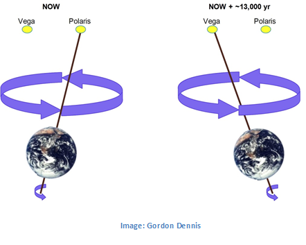 As most people are aware, Earth’s rotational axis is inclined ~23.5° to the plane of the ecliptic, which accounts for the seasons. Currently, the Earth’s rotational axis points almost exactly at Polaris, which is therefore called the ‘pole star’. However, the precession of Earth’s axis has a period of ~26,000 years, so that in around 13,000 years time, Earth’s axis will point at Vega, which will then be the ‘pole star’. Then, in about 26,000 years time, Polaris will again be the ‘pole star’. This is an example of rotational axis precession. The precession of Earth’s rotational axis also accounts for the phenomenon of precession of the equinoxes. The First Point of Aries is one of the two points where the plane of the ecliptic intersects the celestial equator (Davidson, 2020). These are called vernal equinoxes. The first point of Aries was recognized in antiquity in the constellation Aries, but due to precession of Earth’s axial rotation is today located in the constellation of Pisces. Exactly 180° around the celestial equator is the first point of Libra, which today lies in the constellation Virgo. Let’s put that precession cycle into context. The period of precession of Earth’s rotational axis is:  Human civilisations are known to have started ~6,000 years ago. The number of precession cycles during that time is not yet one quarter:  Modern Homo sapiens are believed to have emerged ~200,000 years ago. The number of precession cycles during that time is almost eight:  Earth formed ~4.5 Bn years ago. The number of precession cycles during that time is more than 170,000:  Precession of planetary orbits As was discovered by Kepler, a planet follows an elliptical path as it orbits the Sun. The point at which the planet makes its closest approach is known as periastron. For many years, it could not be explained by Newtonian theory that the periastron of Mercury does not always occur at the same place in the Mercury’s orbit. This is because the orbit itself is subject to precession, so that over a period of time periastron occurs at a point further around the orbit. This was established by careful observation in the nineteenth century. Since Mercury is the planet orbiting closest to the Sun, the precession of Mercury’s orbit is higher than any of the other planets. 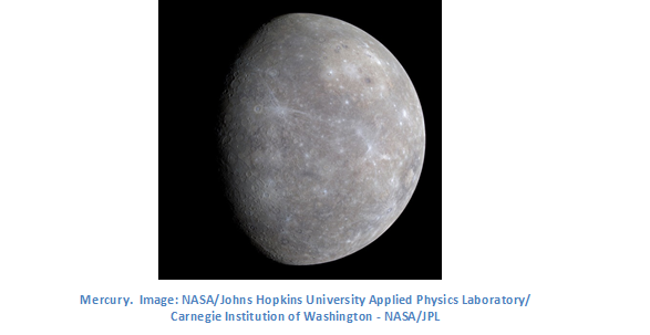 How orbital precession works is illustrated in the diagram below. 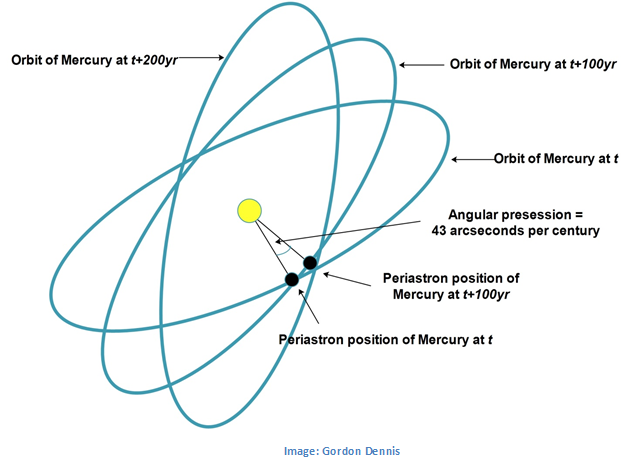 PLEASE NOTE that a) this diagram is looking at the solar system from ABOVE; b) the diagram is emphatically NOT TO SCALE ; c) also, the orbital eccentricities are GREATLY exaggerated; and d) the angular precession angle is GREATLY exaggerated. Newtonian gravitational theory predicts that the magnitude of the orbital precession of Mercury should be slightly more than half what is actually observed. Although many explanations were produced to account for the observations, none were considered conclusive. Einstein’s General relativity (GR), published in 1917, predicted the rate of orbital precession to be 43 arc-seconds per century. This matched the observations exactly. In turn, let’s put that into context. How long does it take Mercury’s orbit to precess a full 360 degrees? Based on angular measure (Helps, 2020), the answer is approximately 3 million years: 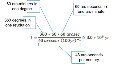 Or, looked at another way: Mercury is estimated to have formed 4.5Bn years ago. That would imply that Mercury’s orbit has completed 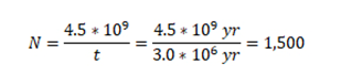 precessions since Mercury’s formation.
This accurate prediction of 43 arc-seconds per century was the first major observational proof that General Relativity is a valid theory. Note that we say a “valid” theory rather than a “true” theory. A scientific theory cannot be proved to be true; it can be showed to accurately account for observations. A scientific theory can only ever be “proved” to be untrue. Later, GR was also able to exactly predict the much smaller orbital precession of Venus (8.6 arc-seconds per century). The second observational evidence pointing to the validity of GR was that gravity of a large mass would “bend” light rays passing close by it - recall John Archibald Wheeler’s ‘mass tells space-time how to curve’ above. This was verified by an expedition lead by Sir Arthur Eddington to observe a total solar eclipse in 1921. But that’s another story. References John Archibald Wheeler: https://phy.princeton.edu/department/history/faculty-history/john-wheeler Mathematics of precession: https://en.wikipedia.org/wiki/Precession Angular size: Helps, L; WMA Blog, May 2020 Celestial equator and plane of the ecliptic: Davidson, B; WMA Blog, May 2020 This year, we celebrate 30 years of the history of the Hubble Space Telescope Here’s the HST itself, and one of its most famous images, taken in 1995. 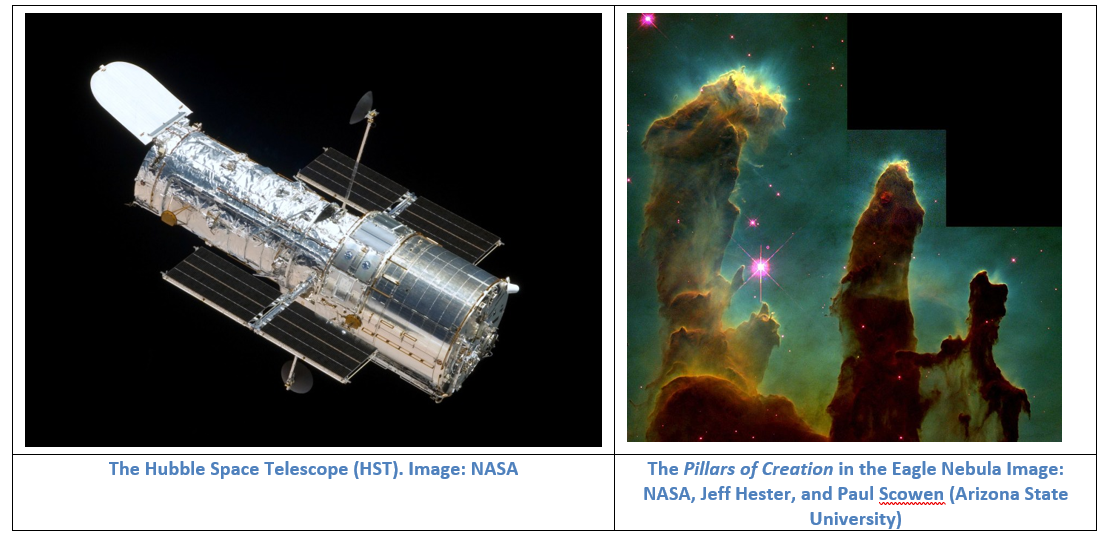 The extent of the universe The HST is named after the American astronomer, Edwin P Hubble, whose observations in the early 20th Century, lead to two, profound discoveries. Looking into these we will also meet several other important characters. Hubble was physically large and imposing. he was a US Army boxing champion, serving at the closing stages of WW1, although his unit did not go into combat. He affected an English accent despite being very much an American. 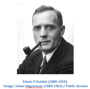 For the first twenty or so years of the twentieth Century, there was great scientific debate about the extent of the universe. Many scientists believed at the time that the whole of the universe consisted of our Milky Way galaxy, and that what were then called “spiral nebulae” were some kind of structure within the Milky Way. Following painstaking observations at the 100 inch Hooker telescope at the Mount Wilson Observatory in California, Hubble and his assistant Humasson established in 1924 that spiral nebulae are in fact remote galaxies in their own right; they are now called spiral galaxies. Hubble’s discovery was made possible by way of an earlier crucial discovery made by Henrietta Swan Leavitt, who worked at the Harvard College Observatory. Leavitt had the task of examining photographic plates to measure and catalog the brightness of stars. 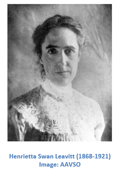 This work led Leavitt to discover the so-called 'period-luminosity relationship' of Cepheid variable stars. Probably the best known Cepheid variable star is Polaris, the current pole star. Leavitt’s discovery was that the rate at which these stars appeared to vary in brightness was directly related to their intrinsic luminosity. This meant that measuring the period of change provided astronomers with the first "standard candle" with which to measure the distance to remote astronomical objects. Hubble used this technique to show that Cepheids in the Andromeda galaxy, M31, was too far distant to be part of the Milky Way Galaxy. It was later discovered that there different types of Cepheid variables, and this meant that M31 is actually twice as far distant as Hubble first calculated. The expansion of the universe Hubble’s second observational discovery was to prove equally profound. It was in fact preceded by a theoretical discovery by Georges Lemaître, a Belgian Catholic priest and professor of physics at the Catholic University of Louvain. Lemaître applied Einstein’s general relativity (GR) to cosmology deriving solutions to Einsteins field equations, giving results that implied an expanding universe. 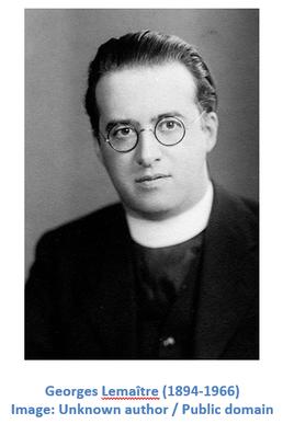 Extrapolating back in time, Lemaître postulated an origin of the universe in what he called a 'primeval atom' – in effect, the “big bang”. This was in 1927, two years before Hubble's publication of his observational findings of expansion of the universe.  An advanced mathematician, Lemaître could hold his corner in intellectual argument with Einstein (no less!). The two met on several occasions, including at the Solvay Conference in 1931. Albert Einstein of course needs no introduction. Einstein published his theory of General Relativity in 1917. Developed from his theory of Special Relativity (published in 1905), GR included an explanation of the phenomenon of gravity. Among other things, GR successfully accounted for variations in the precession of the orbit of Mercury which Newtonian gravitational theory was unable to explain. Einstein had believed that the universe was static, although others (including Alexander Friedman and Georges Lemaître) provided solutions to his equations that indicated that the universe must be either expanding or contracting. 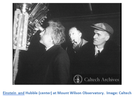 In January 1931, Einstein visited Hubble at the Mount Wilson Observatory where the 100 inch Hooker telescope is located. Einstein, perhaps rather reluctantly, conceded that the expansion predicted by general relativity must be real, added a term called the 'cosmological constant' to his field equations. In later life, he said that this was "his biggest blunder", although today the cosmological constant is now thought by many cosmologists to account for the role of dark energy. Confirming Hubble’s discovery using modern data Hubble's observations, published in 1929, established that the spectra of majority of galaxies exhibit a redshift, showing they are moving away from us, and that the further away they are, the faster they appear to be receding. This became what is now called Hubble's Law and is a cornerstone of modern cosmology. The data plot below shows the plot published in Hubble's 1929 paper. 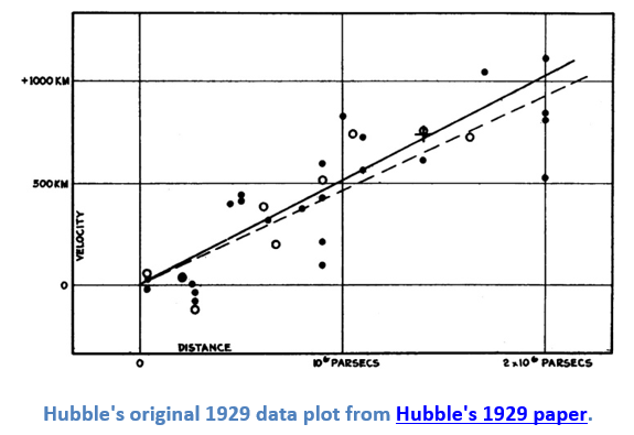 The slope of the trendline indicates the value of what is called the Hubble parameter, H₀, a measure of the velocity of recession of galaxies vs. distance. Hubble's early estimate was that H₀ ~500 km s¯¹ Mpc¯¹ . This was quickly realized to be much too high, as it implied an age of the universe of less than 2 million years, whereas it was known that Earth was much older than this. The plot below has been constructed from modern data in the NASA Extragalactic Database (NED). 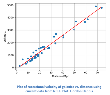 As in Hubble’s work, the plot shows recessional velocities against distances. The red trendline represents H₀. Observations since Hubble's time have refined and reduced the value of H₀ and today the value is thought to be in the range 60-90 km s¯¹ Mpc¯¹ - the exact value is still highly debated in the community. The slope indicates on this plot for this sample of 44 galaxies, H₀ ~64 km s¯¹ Mpc¯¹ .
For Hubble’s confirmation of the extent of the universe and for Hubble’s Law, the Hubble Space Telescope, which has made so many discoveries of its own in its 30 year operation, is named in his honour. So what is Dark Matter? Presumably there must be some kind of exotic particles that constitute Dark Matter (DM). The ‘Standard Model’ of particle physics looks like this: 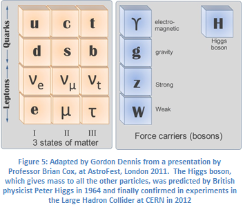 It turns out there are candidates for DM in this model. ‘Neutrinos (the ‘e’, ‘μ’ and ‘τ’ in the leptons group) are DM candidates. Millions of neutrinos pass through the Earth and through our bodies every second, only very rarely interacting with matter. However, neutrinos have an extremely small mass and there are not nearly enough of them to account for the amount of DM required. One group of researchers postulates ‘sterile neutrinos’ which supposedly only interact with other neutrinos, arising when an ordinary neutrino morphs into a sterile neutrino. These results are highly contentious in the community, so neutrinos may only offer a partial explanation. Another theoretical possibility is called a ‘Massive Compact Halo Objects’ (MACHO), a body composed of normal matter whilst emitting little or no radiation. Possible MACHOs include black holes, neutron stars, red dwarf stars and brown dwarf stars, or even planets not associated with any stars. These would be very faint and emit mainly at infra-red wavelengths rather than optical. Some, not completely conclusive observational evidence for MACHOs has been obtained via gravitational micro-lensing observations. Future observations by the upcoming James Webb Space Telescope, which will observe in the infra-red, may detect MACHOs, but there is still a problem. Theoretical studies indicate MACHOs cannot comprise more that 20% of the required dark matter. Add to that the 3% of normal matter we can see, and we still have the question “where is the other 77%?” Another DM candidate is a theoretical, non-baryonic particle named ‘Weakly Interacting Massive particle (WIMP). The characteristics of a WIMP are framed such that if they exist it would answer the question as to what DM is. The theory is that WIMPs ought to interact very weakly with baryonic matter. The inferred distribution of dark matter in our galaxy (i.e. the DM halo) shows a considerable contribution in our location, so as we move through space, we ought to pass through much DM. If DM is made of WIMPs, then we could directly detect the rare interactions between WIMPs and ordinary matter. The existence of WIMPs is allowed under an extension of the standard model of elementary particles called supersymmetry. The first problem with WIMPs is that supersymmetry theory has no observational basis. And the second snag; nobody has detected a WIMP. The last current theory for DM postulates particles named Axions. As with WIMPs, the properties of Axions are framed such that they would account for DM. Because of these properties, axions would interact only minimally with ordinary matter. Axions are predicted to be electrically neutral, have very small mass and very low interaction cross-sections for the strong and weak nuclear forces. This would require modifications to Maxwell’s Equations. Axions would also change to and from photons in magnetic fields. Quite a wish list! Other explanations? Current physics assumes gravity has always acted as it does now; acts the same everywhere; and under all conditions. Suppose that isn’t the case? The leading –though by no means widely accepted - alternative theory to DM is Modified Newtonian Dynamics (MOND) which postulates that under conditions of low acceleration, gravity behaves differently. It also asserts that the inverse square law, while being true over comparatively small ranges such as the solar system, is not applicable over galactic scales. While MOND appears to account for the motions of galaxies without the need for DM, it does not account well for the observed motions within galaxy clusters – reminding us of Fritz Zwicky’s 1933 DM conclusions. MOND also flies right in the face of Einsteins General Relativity, which has passed every experimental test that has been thrown at it since 1917. Most physicists believe DM exists. We do know what DM does. We have little idea about what DM is. Current explanations involve serious modifications of the Standard Model of particle physics, or serious modifications to General Relativity, maybe even both. It’s uncomfortable to think that we don’t know what most of the matter in the universe is. It’s an interesting time to be involved in astrophysics. Acknowledgment The author wishes to acknowledge the assistance of Bob Merritt in the preparation of this article. A question often asked is “what is dark matter?” The answer touches all our understanding of physics - from the very large, at the scale of galaxy clusters; down to the very small, at the level of fundamental particles. Our best answer: we do not know. We know something of what dark matter does. But we don’t know what dark matter is. To be concise, I’ll call dark matter ‘DM’ from now on. “Normal matter” interacts with gravity, and particularly with electromagnetic radiation. In everyday terms, if we heat up normal matter, it will emit electromagnetic radiation. If it shines in the visible region, we can see it with our own eyes. This is exactly what we see when looking at the night sky. In complete contrast, DM does not appear to interact with electromagnetic radiation at all. We see only its gravitational effects. So, what kind of evidence do we have pointing to the existence of DM? Let’s look at just three of the many pieces of evidence for the existence of DM. Clue 1: Motion of galaxies in galaxy clusters The first person to postulate the existence of DM was Swiss astrophysicist Fritz Zwicky, in 1933. Zwicky spent most of his life at Princeton and his observations showed that the gravitational attraction between all the visible matter in the Coma galaxy cluster could not account for the observed velocities of the individual galaxies. 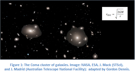 The galaxies are moving so fast that they would exceed the escape velocity of the system (as shown in the inset equation) and would therefore fly apart. The cluster of galaxies would not exist, whereas we can see it plainly using telescopes. Zwicky concluded that there must be much more mass than could be seen visually. Since this missing mass is invisible, Zwicky called it “dunkle materie”- DM. And it was not just a little missing mass – it was a massive amount, many times the mass of the visible matter. At the time, many scientists were openly sceptical of this idea. Clue 2: Rotation Curves of spiral galaxies In the solar system with its eight planets orbiting the Sun, the innermost planet Mercury orbits faster than the second planet, Venus. In turn, Earth orbits slower, Mars slower still and so on. This is called Kepler’s second law, or Keplerian motion, after Johannes Kepler, and it was confirmed later by Sir Isaac Newton. Theory indicates that any system where the majority of the mass is at the centre – as with the solar system – will have a rotation curve like this: 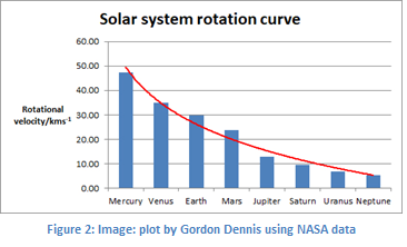 In 1975, Vera Rubin, an astronomer at the Carnegie Institution of Washington and her colleague Kent Ford announced the surprise discovery that most stars in spiral galaxies orbit at roughly the same speed, rather than showing Keplerian motion - these galaxies showed a so-called flat rotation curve. The implication of this is that galaxy mass is distributed approximately linearly with radius well beyond the location of most of the stars. The results suggest that at least 50% or more of the galaxies mass is contained in a DM halo around the galaxy extending to a radius of 100kpc or more. The diagram below shows the rotation curve of our own Galaxy, the Milky Way: 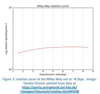 From this data, at least out to 8.5kpc, where our Sun lies, the rotation curve is flat, rather than Keplerian; evidence for DM. Clue 3: Gravitational lensing Gravitational lensing – the bending of space time due to large masses, which causes light rays to appear to bend was predicted by Einstein’s General Relativity in 1917. 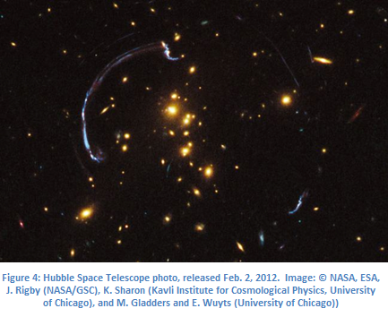 The blue arcs in Figure 4 show the gravitationally lensed image of a galaxy 10 billion light-years away as it appears through the gravitational lens around the galaxy cluster RCS2 032727-132623 about 5 billion light-years away. However, the amount of lensing is too strong to be accounted for by the mass of normal matter in the foreground galaxy. The mass required is much larger: further evidence for DM.
So what is DM? Come back in a couple of weeks for a possible answer...... IF ONLY WE KNEW! As we all do know, forecasting is always difficult, especially of the future. In a maritime climate like ours it’s even harder. In Earth’s atmosphere, most of what we refer to as ‘weather’ takes place at the lower level where we all live – the troposphere. Above this lies the stratosphere. The boundary between the troposphere and the stratosphere is called the tropopause. The precise height of this region depends on our latitude and the timer of year (i.e. where the Earth is in its orbit). In the lower stratosphere, there is a very dynamic wind system known as the jet stream which has a strong influence on our weather down in the troposphere. Jet stream winds can regularly reach over 100mph and are a reason why it can take less time to fly west to east over the Atlantic than it takes to fly east-west. In the images below, the red plots show the strongest jet stream winds. You can obtain a jet stream forecast up tom 10 days into the future at https://www.netweather.tv/charts-and-data/jetstream As a rule of thumb, if the jet stream winds are:
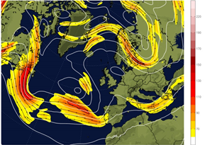
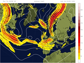
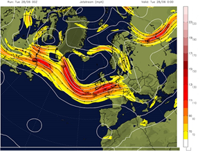 These are not infallible rules, but do give a strong indication to help plan your observations.
|
AuthorWMA members Archives
July 2024
Categories |
 RSS Feed
Proudly powered by Weebly